Chi-Square Test

Chi-square (χ2) is used to test hypotheses about the distribution of observations into categories with no inherent ranking. It compares observed counts with those expected under the null hypothesis (the claim that only chance is at work). The formula is χ² = Σ (O − E)² / E.

What Is a Chi-Square Statistic?

The Chi-square test (pronounced Kai) looks at the pattern of observations. It tells us whether certain combinations of the categories occur more often than we would expect by chance.

That expectation takes into account the total number of times each category occurred.

It looks for an association between the variables. We cannot use a correlation coefficient to look for the patterns in this data because the categories often do not form a continuum.

There are three main types of Chi-square tests. Tests of goodness of fit ask whether one variable matches a specified distribution. The test of independence asks whether two variables are associated.

The test for homogeneity asks whether one variable is distributed the same way in several populations. All three tests share one formula for the test statistic.

These tests compare observed sets of data with theoretical, or “expected,” sets of data. The expected data align with the null hypothesis, the default claim that only chance is at work.

The table below compares the three tests.

Test	Question	Data collected	Degrees of freedom
Goodness of fit	Does one variable follow a specified distribution?	One sample, one categorical variable	Categories − 1
Independence	Are two variables associated?	One sample classified on two variables	(Rows − 1) × (columns − 1)
Homogeneity	Is one variable distributed the same way across populations?	Several independent samples, one categorical outcome	(Rows − 1) × (columns − 1)

What is a Contingency Table?

Contingency tables (also known as two-way tables) are grids in which Chi-square data is organized and displayed. Each cell counts the cases in one combination of two categorical variables, which sort cases into named groups such as gender or sport preference.

They provide a basic picture of the interrelation between two variables and can help find interactions between them.

Each Chi-square test uses two contingency tables. One holds the observed counts (see Fig. 1). The other holds the expected counts (see Fig. 2).

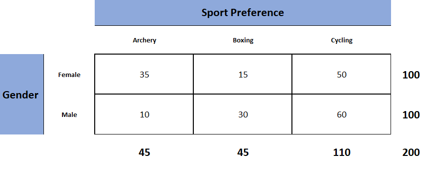
Figure 1. Observed table (which contains the observed counts).

To obtain the expected frequency for any cell, multiply the row total by the column total for that cell. Then divide the product by the total number of cases in the table. This assumes the two variables are independent.

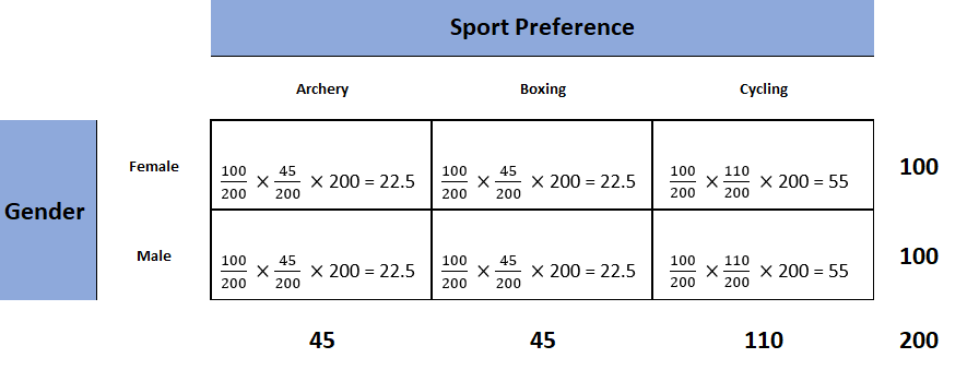
Figure 2. Expected table (what we expect the two-way table to look like if the two categorical variables are independent).

To decide if our calculated value for χ2 is significant, we also need the degrees of freedom (df) for our contingency table. Calculate it with this formula:

df = (rows − 1) × (columns − 1)

Degrees of freedom count the cells that can vary freely once the row and column totals are fixed. A 2 × 2 table has one degree of freedom, and a 3 × 3 table has four.

Formula Calculation

The chi-square formula compares each observed count with its expected count.

χ² = Σ (O − E)² / E

Each symbol stands for one thing:

• χ²: the chi-square statistic.
• Σ: add up the results across every cell of the table.
• O: the observed count in a cell.
• E: the expected count in that cell if the null hypothesis were true.

Each part of the formula has a job. Subtracting E from O gives the gap between what you saw and what chance predicts. Squaring removes the sign. Excesses and shortfalls then both count as misfit.

Dividing by E scales each gap to the noise expected in that cell. A gap of ten matters a great deal when only 20 cases were expected. It matters almost nothing when 2,000 were.

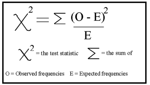
Calculate the chi-square statistic (χ2) by completing the following steps:

1. Calculate the expected frequencies and the observed frequencies.
2. For each observed number in the table, subtract the corresponding expected number (O − E).
3. Square the difference (O − E)².
4. Divide the squares obtained for each cell in the table by the expected number for that cell, (O − E)² / E.
5. Sum all the values for (O − E)² / E. This is the chi-square statistic.
6. Calculate the degrees of freedom for the contingency table using the following formula: df = (rows − 1) × (columns − 1).

Next, check whether your χ2 value is higher than the critical value for your degrees of freedom. The critical value is the cut-off a result must exceed to be significant at your chosen level.

Most statistics books print a χ2 table at the back. If your value is higher, the result is significant at that level.

Worked Example: Gender and Sport Preference

Suppose 100 women and 100 men each choose a favourite sport. Observed counts appear below, with expected counts in brackets.

	Archery	Boxing	Cycling	Total
Women	35 (22.5)	15 (22.5)	50 (55)	100
Men	10 (22.5)	30 (22.5)	60 (55)	100
Total	45	45	110	200

1. Expected count: Multiply the row total by the column total, then divide by N. For women and archery, 100 × 45 / 200 = 22.5.
2. Contribution: Work out (O − E)² / E for each cell. For women and archery, (35 − 22.5)² / 22.5 = 6.94.
3. Chi-square: Add the six contributions to get χ² = 19.80.
4. Degrees of freedom: (2 − 1) × (3 − 1) = 2.
5. Decision: The critical value at .05 is 5.991, and 19.80 also beats the .001 value of 13.816. So p < .001.

The null hypothesis of independence is rejected. Gender and sport preference are associated in this sample: women favour archery more than chance predicts, and men favour boxing.

The test shows an association, not a cause. A report would read: χ²(2, N = 200) = 19.80, p < .001, V = .31 (V is an effect size, explained below).

Interpretation

The chi-square statistic tells you how much difference exists between the observed count in each table cell to the counts you would expect if there were no relationship at all in the population.

Small Chi-Square Statistic

If the chi-square statistic is small and the p-value is large (usually above 0.05), the observed frequencies are close to those the null hypothesis predicts. This suggests no association, or a good fit.

The null hypothesis usually states no association between the variables being studied or that the observed distribution fits the expected distribution.

In theory, if the observed and expected values were equal, the chi-square statistic would be zero. This is unlikely to happen in real life.

Large Chi-Square Statistic

If the chi-square statistic is large and the p-value is small (usually below 0.05), the observed and expected values are significantly different. In a goodness-of-fit test, the data do not fit the specified model well. In a test of independence, a relationship exists between the variables.

A statistic larger than the critical value is significant. For example, 6.40 on 2 degrees of freedom exceeds the .05 critical value (5.991). It does not exceed the .01 critical value (9.210).

This often leads to the rejection of the null hypothesis.

Effect Size: How Strong Is the Association?

A significant chi-square result tells you an association is unlikely to be chance. It does not tell you how strong the association is. The statistic grows with sample size, so a large sample can make a trivial association significant.

To judge strength, report an effect size, a measure of how large an association is that does not depend on sample size. These are the common choices:

• Phi (φ): For a 2 × 2 table, φ = √(χ² / N). It is the correlation between two binary variables.
• Cramér’s V: For larger tables, V = √(χ² / (N × df*)), where df* is the smaller of (rows − 1) and (columns − 1).
• Cohen’s w: w = √(χ² / N). Cohen (1992) gave .10, .30 and .50 as small, medium and large effects.
• Odds ratio: For a 2 × 2 table, Sharpe (2015) prefers it to φ, because unequal row and column totals distort φ.

For V, the benchmarks depend on df*. Divide Cohen’s values by the square root of df*, as in the table below.

df*	Small	Medium	Large
1	.10	.30	.50
2	.07	.21	.35
3	.06	.17	.29
4	.05	.15	.25

In the sport example, V is .31, so with df* = 1 the association is medium-sized.

Following Up a Significant Result

A significant result in a table larger than 2 × 2 is an omnibus result, meaning an overall test. It does not say which cell departs from expectation.

Residuals are the easiest tool. A standardised residual is the observed count minus the expected count, divided by the square root of the expected count.

• Residuals: Adjusted residuals behave roughly like z-scores, so those beyond about ±2 mark cells that depart noticeably from independence (Sharpe, 2015).
• Stricter cut-off: With many cells, raise the threshold or divide alpha by the number of cells (a Bonferroni adjustment).
• Planned comparisons: Choose 2 × 2 sub-tables before seeing the data, which avoids a post hoc correction (an adjustment made after seeing the results).
• Partitioning: Split the table into independent 2 × 2 sub-tables, using likelihood-ratio statistics, which add up to the total.

In the sport example, the adjusted residual is +4.23 for women and archery and +2.54 for men and boxing, using the counts above. With six cells, the Bonferroni cut-off rises to 2.64. Only the archery cell passes it, so that is the clearest difference.

How to Report

To report a chi-square output in an APA-style results section, always rely on the following template:

χ2 ( degrees of freedom, N = sample size ) = chi-square statistic value, p = p value .

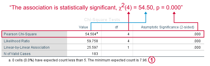
For the example above, the results would be written like this.

A chi-square test of independence showed a significant association between gender and post-graduation education plans, χ2 (4, N = 101) = 54.50, p < .001.

APA Style Rules

• Do not use a zero before a decimal when the statistic cannot be greater than 1 (proportion, correlation, level of statistical significance).
• Report exact p values to two or three decimals (e.g., p = .006, p = .03).
• However, report p values less than .001 as “ p < .001.”
• Put a space before and after a mathematical operator (e.g., minus, plus, greater than, less than, equals sign).
• Do not repeat statistics in both the text and a table or figure.
• Report an effect size, such as Cramér’s V, alongside the test statistic.
• Italicise N, p and effect-size symbols such as V. The Greek letter χ² is not italicised.
• Report any departure from the standard test, such as a Yates correction or Fisher’s exact test.
• For tables larger than 2 × 2, report the follow-up (residuals or contrasts) as well as the overall test.

p -value Interpretation

You test whether a given χ2 is statistically significant by comparing it with a table of chi-square distributions.

Pick the row that matches your degrees of freedom. For a goodness-of-fit test, that is the number of categories minus one. For a table, it is (rows − 1) × (columns − 1).

Check your expected counts too. As a guide, each should be at least five, though Cochran (1954) tolerated a few smaller ones in larger tables.

SPSS reports the p -value for you, in the “Asymp. Sig.” column. If you only have a chi-square value and its degrees of freedom, use the p-value calculator from chi-square.

For a chi-square test, a p-value that is less than or equal to the .05 significance level indicates that the observed values are different to the expected values.

Thus, low p-values (p< .05) indicate a likely difference between the theoretical population and the collected sample. You can conclude that a relationship exists between the categorical variables.

Remember what a p -value is not. It is not the chance that the null hypothesis is true. It is the probability of getting the observed sample distribution, or a more extreme one, if the null hypothesis were true.

A level of confidence necessary to accept the null hypothesis can never be reached.

So you have two options. You either fail to reject the null hypothesis or accept the alternative hypothesis, depending on the calculated p-value. The alternative hypothesis is the claim you accept if the null is rejected.

Chi-Square Critical Values

This table lists critical values at the most common significance levels. Find your degrees of freedom in the left column, then read across.

df	α = .10	α = .05	α = .01	α = .001
1	2.706	3.841	6.635	10.828
2	4.605	5.991	9.210	13.816
3	6.251	7.815	11.345	16.266
4	7.779	9.488	13.277	18.467
5	9.236	11.070	15.086	20.515
6	10.645	12.592	16.812	22.458
7	12.017	14.067	18.475	24.322
8	13.362	15.507	20.090	26.124
9	14.684	16.919	21.666	27.877
10	15.987	18.307	23.209	29.588

A statistic above the value in your row is significant at that level. The further above it falls, the smaller the p-value.

When the null hypothesis is true, the average chi-square value equals its degrees of freedom. A statistic close to its df is what chance alone typically produces. A value several times larger signals misfit.

Using SPSS

Goodness-of-Fit Test in SPSS

Use these steps to run a chi-square goodness-of-fit test in SPSS. This tests whether one variable matches a specified distribution, such as equal expected proportions.

1. Open the test: On the top menu, choose Analyze > Nonparametric Tests > Legacy Dialogs > Chi-square.
2. Choose the variable: Move the variable indicating categories into the “Test Variable List:” box.
3. Equal proportions: To test whether all categories are equally likely, click “OK.”
4. Unequal proportions: Instead, click the “Values” button under “Expected Values.”
5. Enter expected counts: Type the expected count for category one in the box beside “Values” and click “Add.” Repeat for each category in order.
6. Run it: Click “OK.”

Test of Independence in SPSS

Use these steps to run a chi-square test of independence in SPSS Statistics. This tests whether two categorical variables are associated.

1. Open Crosstabs: Choose Analyze > Descriptive Statistics > Crosstabs.
2. Choose variables: Click one variable in the left window, then click the arrow to move it. Select the row variable and the column variable.
3. Request the test: Click Statistics (a new pop-up window will appear). Check Chi-square, then click Continue.
4. Add a chart (optional): Check the box for Display clustered bar charts.
5. Run it: Click OK.

Reading the SPSS Output

SPSS prints several tables for a chi-square test. Check them in this order.

• Crosstabulation: Shows the observed counts, plus the expected counts if you tick “Expected” under Cells.
• Chi-Square Tests: The “Pearson Chi-Square” row holds χ², its df and “Asymptotic Significance (2-sided),” which is the p-value to report.
• Footnote: A line such as “0 cells (0.0%) have expected count less than 5” shows whether the expected-count guide is met.
• Symmetric Measures: Gives φ and Cramér’s V if you tick them under Statistics.

An SPSS p-value of “.000” means p < .001, and you should report it that way. For a 2 × 2 table, SPSS also shows a “Continuity Correction” (Yates’s version) and “Fisher’s Exact Test” (Kim, 2017).

For the goodness-of-fit test, the output shows observed counts, expected counts and residuals. A Test Statistics table then gives Chi-Square, df and Asymp. Sig.

Goodness-of-Fit Test

The Chi-square goodness of fit test is used to compare a randomly collected sample containing a single, categorical variable to a larger population.

This test is most commonly used to compare a random sample to the population from which it was potentially collected.

The test begins with the creation of a null and alternative hypothesis. The hypotheses are as follows:

• Null Hypothesis (Ho): The observed frequencies are the same (except for chance variation) as the expected frequencies. The collected data is consistent with the population distribution.
• Alternative Hypothesis (Ha): The collected data is not consistent with the population distribution.

The next step is to create a table showing how the data would be distributed if the null hypothesis were exactly correct. For each category, multiply the sample size by its hypothesised proportion to get the expected count.

Degrees of freedom equal the number of categories, minus one.

The sample’s overall deviation from this theoretical/expected data will allow us to draw a conclusion, with a more severe deviation resulting in smaller p-values.

Test for Independence

The Chi-square test for independence looks for an association between two categorical variables within the same population.

Unlike the goodness of fit test, the test for independence does not compare one observed variable with a theoretical population. Instead, it compares two variables within a sample against each other.

The hypotheses for a Chi-square test of independence are as follows:

• Null Hypothesis (Ho): There is no association between the two categorical variables in the population of interest.
• Alternative Hypothesis (Ha): There is an association between the two categorical variables in the population of interest.

Next, create a contingency table of expected values. It shows how a data set that aligns perfectly with the null hypothesis would appear.

The simplest way to do this is to calculate the marginal frequencies (the row and column totals). The expected frequency of each cell is its row total multiplied by its column total, divided by the total sample size.

Test for Homogeneity

The Chi-square test for homogeneity is organized and executed exactly the same as the test for independence.

The main difference is in the design. The test for independence looks for an association between two categorical variables within the same population.

The test for homogeneity asks whether the distribution of one variable is the same in each of several populations. The population itself acts as the second categorical variable.

The hypotheses for a Chi-square test of homogeneity are as follows:

• Null Hypothesis (Ho): There is no difference in the distribution of a categorical variable for several populations or treatments.
• Alternative Hypothesis (Ha): There is a difference in the distribution of a categorical variable for several populations or treatments.

The difference between these two tests can be tricky to determine in practice. A reliable rule of thumb is simple. Check how the data was collected.

If the data consists of only one random sample with the observations classified according to two categorical variables, it is a test for independence. If the data consists of more than one independent random sample, it is a test for homogeneity.

Assumptions of the Chi-Square Test

A chi-square result is only as trustworthy as its assumptions. Lewis and Burke (1949) catalogued nine sources of error in how behavioural scientists used the test, and Delucchi (1983) later updated their list. Most are still seen today.

Independent Observations

Each case must appear in the table once, and no case’s category may influence another’s. Three common mistakes break this rule:

• Repeated responses: Counting several responses from one participant.
• Repeated measurements: Treating each measurement from the same person as a separate case.
• Clusters: Sampling siblings or classrooms as if they were individuals.

All three inflate the apparent sample size and make the test too ready to reject. Lack of independence heads Lewis and Burke’s list.

Before-and-after designs need a different test. If the same people are classified twice, use McNemar’s test for paired categories (McNemar, 1947). It uses only the people whose category changed.

A clinical tutorial puts it plainly: each subject contributes to one cell only, and related or repeated groups call for a different test (McHugh, 2013).

Counts, Not Percentages

The statistic is valid only for raw frequencies. Each cell must hold a count of cases, not a percentage, proportion or score (McHugh, 2013).

Cochran (1954) listed using data that are not frequencies among the common misuses.

Percentages quietly change the sample size. A statistic computed on percentages behaves as though N were one hundred. In the gender and sport example above, the true statistic is 19.80. Treating the column percentages as counts gives 42.31 instead.

Categories must also be mutually exclusive and exhaustive. Each case falls in one category only, and the categories cover every case.

Set categories on defensible grounds before collecting data (Lewis & Burke, 1949). Collapsing them after seeing the results changes the test you planned.

Expected Counts and Small Samples

The chi-square distribution only approximates the exact distribution of the statistic. The approximation is poor when expected counts are small. The familiar guide is that every expected count should be at least five.

That figure traces to Fisher’s advice in the 1920s, and Cochran turned it into working rules. Cochran himself regarded five as somewhat arbitrary (Campbell, 2007).

Clinical tutorials restate the rule as at least 80% of cells with an expected count of five or more, and none below one (McHugh, 2013; Kim, 2017).

The expected count is what matters, not the observed one. A cell with zero observed cases is harmless if its expected count is large.

When the guide fails, merge categories on substantive grounds before looking at the results, or choose one of these alternatives:

• Yates’s correction: Reduces each |O − E| by 0.5 before squaring (Yates, 1934). It suits 2 × 2 tables but is conservative.
• N − 1 chi-square: Multiply the statistic by (N − 1) / N. Campbell (2007) found it best for 2 × 2 tables with expected counts of at least one.
• Fisher’s exact test: Gives the exact probability for a 2 × 2 table. It rejects less often than it should and assumes fixed row and column totals.
• Monte Carlo or bootstrap tests: Estimate the p-value from many simulated tables, avoiding the approximation altogether.

The choice can decide significance. Take a 2 × 2 table with counts 7, 2, 3 and 8 (N = 20). Pearson’s test gives p = .025 and the N − 1 test gives p = .029, so both are significant at the .05 level.

Yates’s test gives p = .072 and Fisher’s gives p = .070. Neither is significant.

Say which test you chose before looking at the data, and report the counts.

Critical Evaluation of the Chi-Square Test

The chi-square test is easy to run and easy to misuse. Its strengths and its limits come from one feature: it needs only counts and a null model.

Strengths of the Chi-Square Test

The test works for nominal data, where no test based on means or ranks applies. It handles any number of categories, and the three designs share one calculation.

McHugh (2013) adds that it makes no assumption about the shape of the data and is easy to compute.

It is also everywhere. A survey of all 2008 articles in six psychology journals found 642 reported chi-square tests, about 15% of the 4,248 F, t and chi-square results (Bakker & Wicherts, 2011).

Sharpe (2015) calls it the default choice of applied psychologists for categorical data. Its results are widely understood.

Unlike a t-test, which compares the means of a continuous measure, it compares how cases are distributed across categories. Most psychological data on diagnosis, group membership, choice and behaviour are of that kind.

Limitations of the Chi-Square Test

Four limits matter most in practice:

• Significance, not size: The statistic scales with sample size, so a trivial association can be significant.
• No location: A significant overall test does not say which cells differ.
• Rule of five: The expected-count guide is a convention, and its accuracy varies with table design.
• Independence: Repeated or clustered data break the test, making the sample look larger than it is.

Berkson (1938) argued that no null hypothesis of exact independence is literally true. A large enough sample will therefore make a chi-square test reject nearly anything.

The table shows the effect. The same proportions at different sample sizes give very different p-values. Cramér’s V stays the same.

N	χ² (df = 2)	p	Cramér’s V
20	1.98	.372	.315
100	9.90	.007	.315
200	19.80	< .001	.315
1,000	98.99	< .001	.315

The N = 20 row is arithmetic only, because its expected counts are too small for the approximation to hold.

Categories are also a research decision. The test takes them as given, but researchers decide how many there are and where the boundaries fall.

Coarse or arbitrary categories, such as an age band chosen after seeing the data, can hide differences or create artefacts.

Foundational Study: Pearson (1900)

Pearson (1900) introduced the criterion that became the chi-square test.

The paper was not error-free. It assumed that fitting the expected frequencies to the data cost no degrees of freedom (Stigler, 2008). Fisher (1922) corrected this for contingency tables, which is why the rule above counts (rows − 1) × (columns − 1).

Contemporary Research

Recent work has not changed Pearson’s formula. It has changed the guidance around it: when to trust the approximation, what to do after a significant result, how accurate reporting is, and how to plan samples.

The studies differ in design. An exhaustive calculation or a large audit of published results carries more weight than a simulation of a single proposal.

Do the Expected-Count Rules Hold?

Cochran judged the approximation acceptable when a nominal p of .05 matched an exact p within a narrow band (.04 to .06). Kroonenberg and Verbeek (2018) tested that rule directly.

It is an exhaustive calculation, not a sample, so its p-values are exact. It assumes fixed row and column totals, which many studies lack.

Following Up a Significant Result

From 2012 to early 2014, a search of American Psychological Association journal abstracts by Sharpe (2015) found 13 articles reporting 121 chi-square tests. Thirty-four of those tests had more than one degree of freedom. Nearly all went without a follow-up.

A later simulation found that tests based on adjusted residuals reject more often than they should. The cause is inflated family-wise error, the rising chance of a false positive when many cells are tested.

The authors proposed exact p-values for cell tests, which are more conservative (Shan & Gerstenberger, 2017).

Treat residual thresholds as a guide to where to look. They are not proof that a cell differs.

How Often Are Results Reported Wrongly?

Nuijten et al. (2016) used software to recompute p-values from reported test statistics and degrees of freedom. They checked 258,105 p-values from 30,717 articles in eight psychology journals (1985–2013).

• Articles with extractable tests: 16,695.
• At least one inconsistent p-value: 49.6% of those articles.
• At least one gross inconsistency: 12.9%, about one in eight, where the conclusion changed at the .05 level.
• Trend: Stable or declining over time.

The audit covered t, F, r, χ² and Z tests. Chi-square results can be rechecked in the same way. Report the statistic, degrees of freedom and N in full so any reader can do so.

Planning the Sample

A medium effect (w = .30) on one degree of freedom needs about 88 participants for 80% power at the .05 level. Power is the chance of detecting a real effect.

Abdul Rahman et al. (2025) explain the sample-size formula and provide a free online calculator.

FAQs

References

Abdul Rahman, H., Noraidi, A. A., Hj Khalid, A. N., Mohamad-Adam, A. Z., Zahari, N. H., & Tuming, N. E. (2025). Practical guide to calculate sample size for chi-square test in biomedical research. BMC Medical Research Methodology, 25, Article 144. https://doi.org/10.1186/s12874-025-02584-4
Bakker, M., & Wicherts, J. M. (2011). The (mis)reporting of statistical results in psychology journals. Behavior Research Methods, 43(3), 666–678. https://doi.org/10.3758/s13428-011-0089-5
Berkson, J. (1938). Some difficulties of interpretation encountered in the application of the chi-square test. Journal of the American Statistical Association, 33(203), 526–536. https://doi.org/10.1080/01621459.1938.10502329
Campbell, I. (2007). Chi-squared and Fisher–Irwin tests of two-by-two tables with small sample recommendations. Statistics in Medicine, 26(19), 3661–3675. https://doi.org/10.1002/sim.2832
Cochran, W. G. (1954). Some methods for strengthening the common χ² tests. Biometrics, 10(4), 417–451. https://doi.org/10.2307/3001616
Cohen, J. (1992). A power primer. Psychological Bulletin, 112(1), 155–159. https://doi.org/10.1037/0033-2909.112.1.155
Delucchi, K. L. (1983). The use and misuse of chi-square: Lewis and Burke revisited. Psychological Bulletin, 94(1), 166–176. https://doi.org/10.1037/0033-2909.94.1.166
Fisher, R. A. (1922). On the interpretation of χ² from contingency tables, and the calculation of P. Journal of the Royal Statistical Society, 85(1), 87–94. https://doi.org/10.2307/2340521
Kim, H.-Y. (2017). Statistical notes for clinical researchers: Chi-squared test and Fisher’s exact test. Restorative Dentistry & Endodontics, 42(2), 152–155. https://doi.org/10.5395/rde.2017.42.2.152
Kroonenberg, P. M., & Verbeek, A. (2018). The tale of Cochran’s rule: My contingency table has so many expected values smaller than 5, what am I to do? The American Statistician, 72(2), 175–183. https://doi.org/10.1080/00031305.2017.1286260
Lewis, D., & Burke, C. J. (1949). The use and misuse of the chi-square test. Psychological Bulletin, 46(6), 433–489. https://doi.org/10.1037/h0059088
McHugh, M. L. (2013). The chi-square test of independence. Biochemia Medica, 23(2), 143–149. https://doi.org/10.11613/BM.2013.018
McNemar, Q. (1947). Note on the sampling error of the difference between correlated proportions or percentages. Psychometrika, 12(2), 153–157. https://doi.org/10.1007/BF02295996
Nuijten, M. B., Hartgerink, C. H. J., van Assen, M. A. L. M., Epskamp, S., & Wicherts, J. M. (2016). The prevalence of statistical reporting errors in psychology (1985–2013). Behavior Research Methods, 48(4), 1205–1226. https://doi.org/10.3758/s13428-015-0664-2
Pearson, K. (1900). On the criterion that a given system of deviations from the probable in the case of a correlated system of variables is such that it can be reasonably supposed to have arisen from random sampling. The London, Edinburgh, and Dublin Philosophical Magazine and Journal of Science, 50(302), 157–175. https://doi.org/10.1080/14786440009463897
Shan, G., & Gerstenberger, S. (2017). Fisher’s exact approach for post hoc analysis of a chi-squared test. PLOS ONE, 12(12), Article e0188709. https://doi.org/10.1371/journal.pone.0188709
Sharpe, D. (2015). Chi-square test is statistically significant: Now what? Practical Assessment, Research, and Evaluation, 20(1), Article 8. https://doi.org/10.7275/tbfa-x148
Stigler, S. M. (2008). Karl Pearson’s theoretical errors and the advances they inspired. Statistical Science, 23(2), 261–271. https://doi.org/10.1214/08-STS256
Yates, F. (1934). Contingency tables involving small numbers and the χ² test. Supplement to the Journal of the Royal Statistical Society, 1(2), 217–235. https://doi.org/10.2307/2983604